On Compiling Diagrams to Code
Disclaimer
This essay is not meant to be an academic work.
It contains my opinions from 30+ years of experience in the Software field, running a software consultancy.
As such, references, when included, refer to inspiration and may not be thoroughly researched.
Introduction
This essay discusses a simple compiler that compiles diagrams to executable code.
I believe that diagrams can express certain design elements more easily than textual code. For example, many people draw box & arrow pictures of a desired system on a whiteboard. Such diagrams form a “syntax” for system design. This “syntax” can be made more concrete and can be automatically compiled to code (the old idea of “executable specification” becomes a reality). To make this transition, one needs to “think like a compiler builder” and ask oneself “can I imagine compiling these graphics to code?”. For example, diagrams of stick people and clouds probably cannot be compiled. Diagrams of boxes and arrows can be compiled to executable code, when one creates and follows certain conventions.
In my opinion, diagrams are most useful in the hands of professionals, not children. Most real-world Engineering professions use diagrams, e.g. EE’s use schematics, Civil Engineers use blueprints, etc.
In my opinion, diagrams should not be used to express ideas that are already, sufficiently expressed in textual code, for example
a = b + c;
should not be drawn as a diagram. Such statements communicate perfectly well when written in text form.
Text cannot express - conveniently - a network diagram, for example. A network as text, is a list of components and a detailed “wiring list” between such components and does not communicate the layout of the network to other human readers. For such cases, diagrams excel.
In fact, I believe that a single language cannot express all of the nuances of Software Design. I believe that multiple languages need to be used, e.g. diagrams for software architecture, text code for implementation details, etc. Already, we see many different languages being used in the software creation / distribution pipelines, e.g. bash, npm, gradle, HTTP, CSS, yaml, Docker, etc.
In this essay, I show how to create compilable conventions for drawing such a network diagram and how to compile it to executable code.
The diagrams discussed here are hybrids - diagrams with text annotations. A diagram does not need to express every possible operation. A diagram needs only to express operations that are not conveniently written as text.
Most diagram editors do not make good code editors (DaS - diagrams as syntax). The creation of better DaS editors is discussed in another essay. [Programmers use all 10 fingers, not just a single mouse].
For now, we will use a free editor called Draw.IO (https://www.draw.io/). Draw.IO exhibits the drawbacks of known diagram editors - e.g. one often needs to use a mouse. Draw.IO makes assumptions about the drawing (it begins automagically drawing lines between graphical atoms). Yet, Draw.IO exists, is free and can produce SVG files.
The kinds of diagrams we are concerned with are the kinds of diagrams that Engineers use (e.g. Electrical Engineers (schematics), Civil Engineers (blueprints), etc.).
These diagrams are not meant to make software design easier for novices. They are meant to add further meaning to software designs.
These are technical diagrams.
I believe that technical diagrams for software design have been overlooked due to a bias that assumes that “diagrams are for kids”. In fact, many technical diagrams for software design do exist - on whiteboards in just about every software house. Whiteboard diagrams are, typically, not rigorous enough to be compiled to executable code. I hope to show that compilable technical diagrams are possible and that they do add information to a software project that cannot be easily expressed as text.
The main goal of this essay is to show how modern tools and technologies can be used to implement diagram compilers. We will not emphasise, here, the reasoning behind use of such technical diagrams.
If you already know how a compiler works, you can skip the following section. Note that, I use the “pass” model for compilers instead of the “tree” model. These models are essentially the same, except that the “pass” model uses a pipeline for the compiler and data in the pipeline moves, strictly, from left to right. In the “tree”model of compilation, the tree is traversed downward (top down) then upward (bottom up) - if one is more familiar with the tree model, it might help to imagine that the tree has been flattened and passed from left to right. I find that the pipeline model “keeps things simple” - each pass does exactly one job instead of folding all compiler work into a single textual script based on tree traversal. A major point of simplification is to decompose a problem (in this case a compiler) into subsequent passes (like a bash pipeline) instead of as a data structure.
Classical Compiler Technology
Classical compiler technology splits a text compiler into about four phases, described below.
- Scanner
- Parser
- Semantic Pass
- Coder
Note that this kind of technology is based on “old” ideas, such as : computers are not fast enough to base compilers on backtracking, computers represent text (characters) on the screen, but are too slow and inflexible to represent other glyphs and diagrams on the screen.
The above assumptions led to a great deal of research into textual languages and how to restrict languages to allow for compilation without backtracking.
Efforts such as PEG [Bryan Ford, http://bford.info/pub/lang/peg.pdf], TXL [Cordy, https://www.txl.ca/] show that the above assumptions no longer hold true.
Scanner
The scanner takes in a stream of characters and outputs a stream of tokens.
The main job of a scanner is to ensure that downstream compiler passes do not need to perform string compares.
The scanner performs string matching to determine whether a string of characters in a program match with keywords and operators in the language, or whether strings of characters fall into the class of user-defined identifiers.
Once a match has been recognised, the scanner replaces the matched string with a token that is known to all downstream passes. The main feature of a token is that it can be recognised by downstream passes by a simple numeric or symbolic comparison, instead of a full string comparison.
Depending on the design intent of the compiler-writer, a token may also include information about the token and the matched string. For example, an ID (identifier) token may be a simple integer coupled with a reference to a table entry that contains the actual string of characters, the ID’s type information (updated in later passes), etc.
Early compilers did not contain a scanner pass nor tokens, and they relied solely on streq() operations everywhere. Such compilers ran more slowly.
Early tools, such as Lex […] , read descriptions of strings and converted them into state machines to improve speed, much like the familiar regex(). The techniques of compiling string matchers into state machines are covered in the Dragon Book […].
Parser
The job of a parser is to check that tokens are correctly placed / sequenced to fit the particular language being compiled and to signal errors if the tokens do not form well-formed phrases in the language.
For example in C, the string “(x ==y)”, might be represented by the sequence of tokens (represented by symbolic names):
tokLPar
tokIdent {ref. to table entry for ident “x”}
tokEqualsEquals
tokIdent {ref. to table entry for ident “y”}
tokRPar
In this case, each token, tokLPar, tokIdent, tokEqualsEquals and, tokRpar might be represented as Integers (scalars) and the extra information, enclosed in braces ({}) would signal that tokIdent has some kind of structured information following it.
The string of five tokens, above, form a well-formed Expression in C.
The parser, also, has the job of discarding syntactic sugar and replacing token phrases with shorter token phrases which contain only the information necessary in subsequent passes.
For example, the Parser might re-emit the tokens in an RPN stream as follows:
tokExpression
tokIdent {ref. to table entry for ident “x”}
tokIdent {ref. to table entry for ident “y”}
tokEqualsEquals
Semantic Pass
A Semantic Pass has the job of checking the semantics of program token phrases. The semantic pass doesn’t need to check tokens or the validity of token phrases - these are verified in preceding passes (the scanner and the parser). Checking the semantic validity of token phrases can be a complicated matter, but is simplified by information generated by the preceding passes.
In general, the semantic pass needs to determine the scopes of all variables (subject to scoping rules of the language) and the types of all variable (subject to typing rules of the language).
In declaration-before-use languages, the semantic checker can be collapsed into a single pass, whereas, in languages that do not follow the declaration-before-use rules (and possibly require transitive closures over the complete system), a semantic pass might consist of more than one actual pass.
Specifying declaration-before-use semantics assists the compiler writers, but puts more onus on the users of the language (e.g. to declare objects earlier than strictly necessary).
Thirty years ago, it was considered “reasonable” to off-load such considerations to language users.
Today, with much faster hardware, it seems to me that encumbering the software designer with rules that make compiler-writing easier for the compiler-writer, is a false economy. All efforts should be used to off-load mental strains from the software designers.
Allocation and Coding
After a program (a token stream) has been “certified correct” by preceding passes, the compiler-writing job consists of creating code.
The act of code creation breaks down into, at least, two phases:
- Allocation - figuring out where each variable, constant, parameter and return value is going to end up in the memory space (stack, etc.).
- Choosing code sequences (in the appropriate assembler) that faithfully carry out operations in the higher level language (being compiled).
Allocation
For allocation, one needs to represent data-locations in some manner.
One method is to use a data structure called “data descriptors” [Holt, https://dl.acm.org/citation.cfm?id=24051].
Fraser/Davidson designed RTL [Fraser-Davidson, https://people.well.com/user/cwf/pro/Davidson%20and%20Fraser.20The%20design%20and%20application%20of%20a%20retargetable%20peephole%20optimizer.pdf], the method used in gcc.
Coder
A coder is the final pass in a compiler. Coders are also called “emitters” and “back ends”.
It simply walks the stream / tree and emits code (as assembler text, or binary) for a particular cpu architecture.
Another aspect of coding is “optimisation”. This pass can precede or succeed allocation and emission, depending on design constraints and implementation of various compiler data structures.
Coders often rely on a library known to contain certain operations that will be included at run time ( a “run time” library). The final emitted code is linked with this library.
Coders/emitters/backends make trade-offs for speed vs. code (and data) size.
Coders need to determine which cpu registers will be used. [Note that, in a multi-process environment, each register which might contain data must be pushed onto a stack (to save the value(s)) during context switches)].
Tree-Based Coding
See https://en.wikipedia.org/wiki/Compilers:_Principles,_Techniques,_and_Tools .
Optimization
A very common form of optimiser is a tree-based one. This kind of optimiser is described in [Aho,Ulmann,et al, https://en.wikipedia.org/wiki/Compilers:_Principles,_Techniques,_and_Tools (“the dragon book”)].
A tree-based optimiser can convert a tree into a DAG and can easily reuse code sequences and allocations that appear more than once.
A very simple form of optimisation is “peephole” optimisation. This method executes after the coder phase and looks at the emitted code through a “window” of some number of instructions. It pattern-matches the windowed instruction sequence and replaces matches with “better” code (faster or less space, etc.). Peephole optimisers can be built using very simple tools, like awk.
Run-time Library
In older C compilers, the run time library was called “crt0” (C Run Time zero).
Run time libraries often perform startup and initialisation task, as well as providing routines for certain repetitive code sequences (e.g. floating point) that are better (space-wise) left as libraries instead of full-unrolled code sequences emitted by the coder.
Portability
There has been a fair amount of thought put into creating machine descriptions that reduce cognitive load for the compiler writers. For example, OCG (orthogonal code generation [Cordy, https://books.google.ca/books?id=X0OaMQEACAAJ&dq=bibliogroup:%22Technical+report+CSRI%22&hl=en&sa=X&ved=0ahUKEwjg4Y7a7ZbiAhUMwlkKHfzdD_MQ6AEIMzAC]) allows one to declaratively specify a tree of code sequences based on cpu architecture. The tree(s) specify how to map operations, in some low-level form, into a correct sequence on instructions for a number of architectures.
Backtracking
In the past, it was assumed that a single cpu was expensive and that it needed to be time-shared between users.
In the past, machines were much slower than they are today.
It was “determined” that backtracking was not practical, hence, compilers were designed to conserve speed.
Compiler technology was invented to accommodate speed and determinism. YACC reduced the acceptable set of languages to LALR(1), so that it could implement parsers as NFDAs.
PEG [Bryan Ford, http://bford.info/pub/lang/peg.pdf], TXL [Cordy, https://www.txl.ca/] and Prolog [Clocksin, Mellish, https://link.springer.com/book/10.1007/978-3-642-55481-0] show that backtracking is practical on modern computers. A trend towards more flexible languages has not followed this trend in faster computers.
Drawing Conventions
As it stands, we do not have an off-the-shelf drawing editor.
We use an existing diagram editor plus some conventions that make its output suitable for compilation. We do not check all drawings for correctness and the compiler may fail (or produce incorrect code) if drawings contain features not specified below.
For now, we will use the (free) Draw.IO drawing editor and save the drawings as .SVG files.
For drawings made with Draw.IO, the following conventions are used:
- A Part is drawn as a Rectangle (top-left of General palette) with Text (3rd item on General palette) completely inside the Rectangle. The Text represents the kind (aka, type, class) of the part. There can be multiple Parts with the same kind in a drawing. These are recognised as multiple instances of the same kind of part. Instances are given unique ID’s internally, that are not shown on the diagram (see Figure: 1).
- A Wire is drawn as a “directional connector” (line with arrowhead) (32nd item on the General palette) from one rectangle to another. The connection points are displayed by Draw.IO when the line is dragged near, or across, the boundary of the rectangle.
- A Wire must be a single, contiguous line. It must not be split into multiple line segments. Draw.IO allows one to place multiple “bend points” on a line - this is allowed, as long as the line is not split into multiple segments.
- The beginning of a wire/line is unadorned. The end of a wire is marked with an arrow-head. Events flow from the beginning of a wire to the end. The compiler expects the beginning of a wire to touch the rectangle. On the other hand, arrowheads (ends of the wire(s)) can be +-20 units from the edge of a rectangle. Draw.IO draws lines in way that the beginning touches a rectangle, but draws the end of a line so that they do not touch a rectangle (only the arrowhead touches the rectangle ; it was easier to add a kludge factor to the end of wires than to sort out which arrowheads correspond to which lines ; the kludge factor only applies to arrowhead portion of a line, all other matches are exact).
- A Port is a text box (3rd item on General palette) that is not contained inside the rectangle, but is positioned “near” one end or another of the wire. The Port’s name is a numeral. The range of numerals depends on the compiler. In this POC, Port names start at 0 up to 15. The compiler measures distance from the beginning or end of a wire to unenclosed text. The text closest to the end of a wire is taken to be the index of the Port. Currently, ports are “named” by a numeric index. In the future, the compiler can be changed to accept arbitrary character strings for port “names”. This is not the case, currently (the compiler only understands numeric indices).
- A port with no arrow is an output pin. A port with an arrow-head is an input pin.
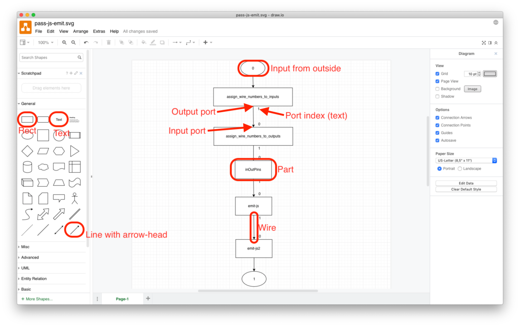
Figure: 1
- Multiple wires can connect to input pins and to output pins. (“Fan out” and “fan in”, resp.). (N.B. FBP allows “fan in” but does not allow “fan out”. The drawings discussed here do not follow all FBP conventions and allow for “fan out”, similar to electronic schematics).
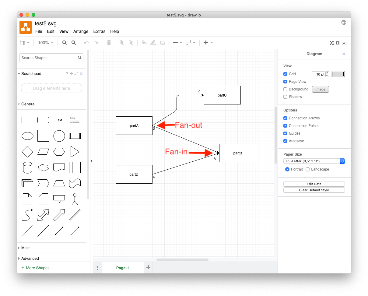
Figure: 2
- Time-ordering is preserved. An event that is placed on a wire arrives at all inputs (in the same schematic) at the same “time”. A wire that is attached to multiple inputs (“fan out”) is, therefore, more “costly” than a wire that connects a single output to a single input (N.B. some care is needed when implementing multiple connection and simultaneous delivery in a preemptive (time-sliced) environment. Fan-out requires that the event be delivered to a group of wires/pins atomically. When time-slicing and/or interrupts are being used, there might be a need for some locking under-the-hood to guarantee atomic delivery of events to implement fan-out) [The current PoC performs atomic delivery implicitly]. It is, also, implementation-dependant as to what happens when non-scalar events are fanned out (e.g. an implementation can refuse to support non-scalar fan-in, or it can implement under-the-hood non-scalar event copying).
- Inputs from the outside and outputs to the outside are drawn as ellipses with a port number fully enclosed inside the ellipse.
- [Dots are currently unimplemented, since they are just “syntactic sugar” for fan-in and fan-out at ports]. Dots, drawn as small black circles (Draw.IO ellipses that are round, and filled with color black).
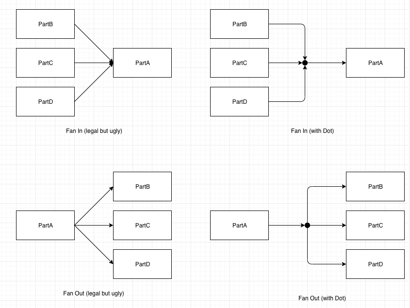
Figure: 3
Multiple wires can connect to a dot. Dots are “one-way”. A dot can have many arrow-heads pointing into it and only one wire emanating from it, or, one arrow-head pointing into it, and many wires emanating from it. A dot must not have multiple inputs and multiple outputs. The meaning of dots are (1) many inputs (arrow-heads) pointing in and one wire pointing out means that all of the incoming wires are compressed down into the single output (all inputs go the same place as the single output) and (2) one input and many outputs means that the input is split (copied) to all of the outputs simultaneously. - Composite Parts — parts which are made up of a schematic referring to other parts — are managed manually. A composite Part consists of a drawing (a schematic) containing boxes, arrows, ellipses and dots. When a composite diagram is compiled and run, it is assumed that the children parts all exist (the compiler does not currently check for this). Composite parts can be nested hierarchically, each part on its own schematic.
- Draw.IO must be instructed to save the drawing as an .SVG file (change the name to <name>.svg before saving).
- Hints: Draw wires first, then annotate the wires with port numbers. When moving or re-drawing a wire, move existing port numbers far away from the rectangle and connect the wires, then move the port numbers back into position. Draw.IO allows wires to connect to Text, but this is not what we want - wires must be connected to rectangles. When a port number is left in place, while moving an reconnecting a wire, Draw.IO might connect the wire to the rectangle or to the port number - it remains visually unclear as to which connection is made.
The Algorithm
To describe the algorithm for compiling 2D drawings to code, I will use the “standard” four-pass model for compiler-building from the 1D text language paradigm. A final version of the diagram compiler might use a separation that is different from the four-pass model, but it appears that the four-pass model might make for a simpler explanation at this time. In fact, the current compiler has about twenty “passes”, grouped into four larger (composite) parts.
Draw.IO outputs drawings in various formats. bmFBP drawings use the conventions discussed earlier and are saved as .SVG files.
In this algorithm, we always add facts to the factbase. In principle, it is possible to remove facts from the factbase, but such action is not necessary - downstream passes match only for the facts they are “interested in”. Superfluous facts are skipped over and their only effect is to slow down the pattern matching (backtracking). In the diagrams we have compiled, slow-down is not noticeable and pruning facts is not necessary.
Scanner
The scanner pass simply strips and discards unused SVG information and outputs a Prolog factbase.
Each fact appears on separate lines in the format
relation(subject,object).
Where the relation is some sort of relationship (declared in head.pl and tail.pl), the subject is a unique id and the object is a unique id (of some other graphic object) or a piece of data (usually an integer or floating point number).
The scanner recognises and emits four kinds of graphical objects:
- Rectangles
- Ellipses (with no-fill-color or black-fill-color)
- Text
- Directional lines (with arrow-heads).
As it stands, the POC compiler takes a component-name from the command line and emits a fact
component('name').
(The component name should, in the future, come from the IDE, sent in through an ellipse input).
For every line, we know that the line has a sink port (its beginning — where events are consumed) and a sink port (its end, where events are emitted). “Source” means that events “come from” the port. “Sink” means that port accepts events as input. On children parts, “sink” ports are inputs while “source” ports are outputs. On the parent part (the drawing itself), the input port “sources” events (from the outside) while the output ports “sink” events (emit events to the outside). We can calculate the bounding box for each port using a fixed constant (e.g. 20) for its size in x and y. In a later pass, we will add more bounding box for other graphical elements. Emit a set of facts (where “eltype” means “graphic element type”):
line(new-id).
source(line-id,begin-id).
eltype(begin-id,'port').
bounding_box_left(begin-id,nnnn).
bounding_box_top(begin-id,nnnn).
bounding_box_right(begin-id,nnnn).
bounding_box_bottom(begin-id,nnnn).
sink(line-id,end-id).
eltype(end-id,'port').
bounding_box_left(end-id,nnnn).
bounding_box_top(end-id,nnnn).
bounding_box_right(end-id,nnnn).
bounding_box_bottom(end-id,nnnn).
For every rectangle, output its ID, eltype (‘box’) and geometry x/y/width/height.
rect(rect-id).
eltype(rect-id,'box').
geometry_x(rect-id,nnnn).
geometry_y(rect-id,nnnn).
geometry_w(rect-id,nnnn).
geometry_h(rect-id,nnnn).
1For every text graphical item that contains only numerical digits, emit it’s id, the “text” as a number and its geometry.
text(text-id,nnnn).
geometry_x(text-id,nnnn).
geometry_y(text-id,nnnn).
geometry_w(text-id,nnnn).
geometry_h(text-id,nnnn).
For every text graphical item that contains any non-numerical characters, emit it’s id, the “text” as a string and its geometry. (Currently, the compiler uses strings for part kinds and numbers for port indices. When creating the initial factbase, it is “easy” to differentiate between strings and numbers. Prolog can easily differentiate between these two types using the hint that strings are quoted and numbers are not. This differentiation helps downstream passes, by making it obvious what the text contains, since the downstream passes do not need to perform differentiation, since it is already done).
text(text-id,'string').
geometry_x(text-id,nnnn).
geometry_y(text-id,nnnn).
geometry_w(text-id,nnnn).
geometry_h(text-id,nnnn).
For every arrow-head, emit it’s id and an (x,y) pair that corresponds to the “tip” of the arrow-head.
arrow(arrow-id).
arrow_x(arrow-id,nnnn).
arrow_y(arrow-id,nnnn).
(As can be seen, the scanner is relatively “simple” and does little work. The last two passes inside the scanner - plsort and check_input - do almost “nothing”. Plsort simply sorts the factbase, since Prolog requires that all rules with the same name be contiguous, and “check_input” does an incoming sanity check to check that the factbase is clean. In this case, we simply rely on Prolog to signal bad rules. “check_input” simply reads then writes out the factbase. If prolog signals no errors then the sanity check is deemed to have succeeded. In the future, check_input might be extended to check more details.)
Parser
In this POC, “parser” does most of the work, consisting of 9 passes (each one fairly simple):
- Calculate bounding boxes for Rects and Text, insert the bounding box facts for each item into the factbase. This pass adds four kinds of facts to the factbase: bounding_box_left, bounding_box_top, bounding_box_right and bounding_box_bottom, each with an ID and a number. [calc_bounds].
- For every rectangle, find a graphical text item that fits inside the box (its kind (aka type or class)). For every such text item, mark it as “used” (simplifies searching in later passes). The “kind” is marked with a kind(id,text-id) fact and a used(id) fact. [add_kinds].
- For all text items that are not marked as used, create an unassigned fact. This is a superfluous operation, but makes downstream passes “easier” - unassigned means that the item is text and that it is not marked as being used (i.e. used as a kind name of a rectangle). [make_unknown_port_names].
- Create a center (x,y) for every port and every unassigned text item. [create_centers].
- For every port, calculate the distance to every unassigned (text) item. We stay true to the idea of making every fact a triple (and only a triple). This requires the use of an indirect fact called join which joins a port to each calculated distance for each unassigned. In “normal” Prolog, we could simply list the PortID, the TextID and the Distance in a single fact (instead of using indirection via join). [calculate_distances].
- For every Port, make a list of distances to unassigned text. Choose the minimum distance in the list, then create a pair of facts that connect the PortID to the TextID (portIndex) and another fact that points “backwards” from the TextID to the PortID (portIndexByID). [For the sake of future revisions, also create another pair of facts using string name (portName, portNameByID) - not strictly needed by this algorithm.]. [assign_portnames].
- Mark every port as a sink or a source, as appropriate. [markIndexedPorts].
- To allow fan-out and fan-in, ports can overlap one another (see figure 1.3). For every group of overlapping ports, only one port actually has an index assigned to it. Propagate the index to all other overlapping ports. [coincidentPorts].
- For every port, calculate which Part (a rectangle ‘box’) the port intersects with and insert a new parent fact relating the port to its parent. [match_ports_to_components]. Clearly, the semantic pass should check that each port intersects one and only one Part.
At this point, the algorithm is almost finished - a diagram, following conventions as described earlier, has been entered into the factbase and the factbase contains sufficient information to produce code. As can be seen, the algorithm is very simple. A production version of this algorithm would include more semantic checks.
Semantic Pass
The semantics pass checks various design rules. If any check doesn’t pass, it should abort code generation. At present, there are only two passes built as examples of semantic checking - sem_partsHaveSomePorts (every Part must have at least one port) and sem_allPortsHaveAnIndex (every port must have a numeric index (this index is used during code generation)). The semantic pass could (should) have many more checks, but as can be seen, using backtracking pattern matching over the factbase makes piece-wise semantic checking “easy”. In fact, the semantic checks could be spread throughout the compiler and abort compilation at its earliest convenience.
Code Emitter
The code emitter walks the factbase and creates a file of text for a given language. In this case, a JSON table is emitted for JavaScript. There are currently 5 steps to doing this:
- Create a “wire number” for every wire. Since every wire is connected to one source and one sink, as per the diagram conventions, we arbitrarily walk the sinks and assign wire numbers. For every sink port, match the wire(s) that it is connected to, and assign a wire number, starting with 0 and increasing by 1 monotonically. Keep a count of the number of wires on a given diagram. [assign_wire_numbers_to_inputs].
- For every source port, match the wire(s) that connect to it, then associate the wire number with the wire(s). Use the already-chosen wire number from step one, from the sink attached to a given wire.
- For every sink Port on every Part, create two facts - the inputPin and wireIndex facts. Do the same for every source Port on every Part (outputPin and wireIndex). [inOutPins].
The algorithm for handling ports is a subset of the main algorithm. Port handling is described below.
Scanning
During scanning, we know that each line has a port at its beginning and a port at each end. We don’t yet know what the port is attached to or if it is an N/C (no connection.
During scanning, we attach a port to each end of the line, and, since all lines are arrows, we can also assign a “direction” (source (output) or sink (input)) during this pass. For example, each line has the following facts entered into the factbase: an new id for the line, a source port (output port), a bounding box for the port based on (x1,y1) of the line and a sink port (input port).
The bounding boxes for the ports are “invented” at scan time. These “invented” ports are made to be 40 pixels on all sides.
The facts appear in the factbase as:
line(new-id).
% port at line beginning
source(line-id,begin-id).
eltype(begin-id,'port').
bounding_box_left(begin-id,(x1 - 20)).
bounding_box_top(begin-id,(y1 - 20)).
bounding_box_right(begin-id,(x1 + 20)).
bounding_box_bottom(begin-id,(y1 + 20)).
% port at line end
sink(line-id,end-id).
eltype(end-id,'port').
bounding_box_left(end-id,(x2 - 20)).
bounding_box_top(end-id,(y2 - 20)).
bounding_box_right(end-id,(x2 + 20)).
bounding_box_bottom(end-id,(y2 + 20)).
Parsing
In “make_unknown_port_names”, we find all pieces of text that have not yet been associated with any Parts (rectangles). This includes all text that consist only of digits (i.e. port indices). Each of these pieces of text are given an “unassigned(TextID)” fact.
In “create_centers” we assign “center_x(ID,N)” and “center_y(ID,N)” facts to all unassigned pieces of text and all ports (eltype(ID,port)).
In “calculate_distances” we create a distance vector from every port to every unassigned piece of text (this is inefficient but works in the POC. Maybe there is a better way). In this particular case, I decided to create a new Object called a Join with a unique ID. A unique “join_centerPair” is created for every Port. Each join_centerPair has two facts created for it - “join_distance(Join_centerPairID, TextID)” and “distance_xy(Join_centerPairID,Distance)”. The former connects the Port to one unassigned piece of text and the latter gives the distance between the Port and the one unassigned piece of text. Again, there might be more efficient ways to express this connection.
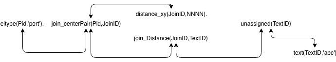
Figure: 4
In “assign_portnames” (finally), for each port, we find the unassigned piece of text that is closest to the given port and associate the port and the text via a portIndex fact. Furthermore, we associate the text with a back-pointer fact “portIndexByID”. Historically, we create two more facts that mirror this two-way association with “portName” and “portNameByID” for pieces of text that are not numeric. Historically, we started out with textual port names. Later, we discovered that every port needs an index (for the coder pass) and made a new convention that insists that every port must have an index and that only some ports may have names. We currently ignore textual port names. In the future, I may return to using textual names for ports while automatically creating numeric indices for ports.
In the two-Part pipeline, “markIndexedPorts” and “coincidentPorts”, I implement fan-out and fan-in. I find all ports that overlap each other and assign the same index to all of those Ports.
The Part “mark_directions” is a no-op for this POC compiler. In some editors, the direction of lines is not specified. In such cases, lines might be made up of segments with no direction associated with them. In such cases, the compiler needs to trace all connected segments to find the ultimate beginnings (sources) and ends (sinks) of the lines and create a virtual directed line between the beginning and end Ports. In this POC, we use Draw.IO, and use the convention that all lines (wires) use Draw.IO’s arrows. Draw.IO arrows already provide direction information, so “mark_directions” is a no-op in this case.
The Drawing Compiler
This section documents the actual facts and passes used by the current POC (proof of concept) compiler.
These choices might not be the best ones, since understanding of the architecture grew over time, but they do represent the contents of the current POC.
Basic Concepts
The basic requirements for compiling a diagram are:
- To “arbitrarily” choose a set of graphical “atoms” which can be used to draw the diagrams for the language.
- Then, use pattern matching and backtracking to infer new, semantic information which builds a knowledge base (some kind of data structure) that represents the interesting details within the diagram.
- Finally, convert the inferred information into some other text language, which is then compiled into executable code in the usual way, using existing compilers and tools.
At first, this may seem difficult or impossible. One can use the method of “divide and conquer” to create ridiculously small components, to produce a working diagram compiler.
I have concluded that no single programming language can do everything that is required, to solve an actual real-world problem. Several “design principles” come from this conclusion:
- Use a paradigm and a language that is most suited to the task(s) at hand.
- Don’t over-design. Create only what is needed to solve the problem. Abstraction and generalisation are over-sold. If done too early (e.g. before some 3 iterations on the solution), abstraction is a bad idea that wastes time and usually doesn’t solve the problem at hand. A corollary is: code reuse is a bad idea, design (architecture) reuse is a better goal - code is (can be) cheap, thinking is hard. Reuse “thinking”. Refactoring is a symptom of poorly-expressed design. If you feel a need to refactor code (instead of just throwing it away), then you are probably doing something else wrong.
- Don’t build the Design into the program - encapsulate the Design and pull it out of the code. Spaghetti Design is worse than spaghetti code.
- Don’t generalise, just get the job done. Code libraries bring other problems into the mix, which detract from getting the job done, as we’ve seen over the decades. Making it possible to reuse the Design (the thinking time, e.g. patterns) results in better use of human resources than taking the time to abstract code and to make it a part of a library.
The above principles have led to an extremely simple diagram language, as discussed below.
Graphical Atoms
In this diagrammatic language, we simply need about two (2) graphical objects - straight lines and text. This diagrammatic language consists of
- boxes and
- arrows.
I will show that a language as simple as this, can result in useful expression of software concepts that cannot be done with text alone (esp. when the boxes represent asynchronous actions, not synchronous ones).
The next step up is to infer rectangular boxes. Rectangular boxes can be inferred from a diagram by pattern matching straight lines and discovering lines that have common (x,y) end points.
Many drawing tools provide rectangular boxes, so we can simply add them to the list above. In this POC (proof of concept), we are using Draw.IO. Draw.IO provides rectangles as atomic graphical objects, hence, we can avoid inferencing rectangles. We extend the above list to three (3) items -
- straight lines,
- text, and
- rectangular boxes.
Draw.IO also provides straight lines with arrow-heads as primitive graphic atoms. We will need to know the “direction” that lines point in, hence, we extend the the above list to four (4) items:
- straight lines,
- text,
- rectangular boxes, and
- arrow-heads.
Another diagrammatic language, say one for expressing StateCharts, might use another completely different set of graphical primitives (e.g. curved lines, text, ellipses, dotted ellipses, callouts), but, using the “do not over design” principle, above, we will ignore these other atoms for now. Building a compiler for StateCharts is another project (and, it has been done in the past).
FactBases
The “ideal” data structure for the compiler is one that implies no structure (!) to the data.[1] One such data structure is the factbase[2] .
A factbase is an unordered collection of facts.[3] A fact is a simple 3-tuple that contains a Subject, an Object and a Relation between them.
In Lisp, a fact might be represented as
(relation subject object)
In Prolog, a fact might be represented as
relation(subject, object).
To keep things ridiculously simple, we can implement a factbase as a file, with one fact per line and with empty lines being ignored. We append new facts to the front or to the end of the file (whichever is easiest - we don’t actually care, since the factbase is unordered).
In this example, the most basic factbase would contain only the four graphical atoms plus geometry facts that describe their X and Y positions on the diagram plus width and height information (if appropriate). For example, a simple factbase might be:
text(id1,’’).
text_string(id1,’hello’).
text_x(id1,100).
text_y(id1,200).
Here, ‘id1’ is some unique ID for the text. The first line “declares” the existence of a piece of text on the diagram. The rest of the lines all refer to the same ID (id1) and specify properties of the text e.g. the actual string of characters of the text, the (x,y) coordinates of the text.
Facts are very similar to N-tuples found in the semantic web, etc. A factbase is very similar to triple-stores. Triple-stores and n-tuples are more general than what is needed for a diagram compiler, so they will be ignored for now.
Pattern Matching & Backtracking
One operation that will be used repeatedly is pattern matching for inferring new information within the factbase.
Prolog is a language that expresses both of these operations conveniently, and Prolog is freely available.
I use gprolog in this project.
I assume that mini-Kanren (micro-Kanren) could be used (but, I haven’t explicitly tried that idea yet ; micro-Karen is available in Scheme, Clojure and Haskell, among other languages, and its use is detailed in the book “The Reasoned Schemer”).
As an example of what we might use Pattern Matching & Backtracking for is to infer that a rectangle is formed out of four lines (not that, if we use Draw.IO, we won’t actually need to do this):
line(id2,’’).
line_x1(id2,10).
line_y1(id2,10).
line_x2(id2,20).
line_y2(id2,10).
line(id3,’’).
line_x1(id3,20).
line_y1(id3,10).
line_x2(id3,20).
line_y2(id3,20).
line(id4,’’).
line_x1(id4,20).
line_y1(id4,20).
line_x2(id4,10).
line_y2(id4,20).
line(id5,’’).
line_x1(id5,10).
line_y1(id5,20).
line_x2(id5,10).
line_y2(id5,10).
The above factbase describes one rectangle as a set of four lines (id2, id3, id4, id5). [X’s increase to the right, Y’s increase downwards, in this coordinate system].
Pattern matching can be used to infer the rectangle by checking the endpoints, for example, the end-point of id2 matches the beginning-point of id3 and so on, all the way around.
When we find such a closed rectangle, we insert a new set of facts into the factbase, for example:
rectangle(id6,’’).
rectangle_center_x(id6,15).
rectangle_center_y(id6,15).
rectangle_width(id6,10).
rectangle_height(id6,10).
It is simple-enough to write rules in Prolog, that pattern-match and backtrack to find all such rectangles in the factbase.[4]
In earlier days of computing, it was considered impractical to use backtracking in this way. Numerous methods were developed to pattern match streams of characters (e.g. Lex to match strings of characters using state machines, Yacc to match strings of tokens using state machines). These methods tended to restrict the kinds of sequences (languages) that could be recognised (e.g. Yacc could pattern match LALR(1) grammars and would raise errors if the incoming language did not conform to LALR(1)).
Modern computers (2010 +) and Prolog engines make backtracking practical and quick.
Using successive pattern matches, it is possible to infer a great deal of information about diagrams and to use this information to produce code from a diagram.[5]
As an example, one version of this notation denoted Ports as small squares positioned on the edge of larger Parts. The inference was done using small steps - (1) pattern match ALL rectangles (and squares) (2) find all squares (3) find all squares that intersect the edges of bigger rectangles, and declare (by adding facts to the factbase) that the small squares are Ports and which rectangular Parts they belong to, e.g.
…
port(id31,’’).
parent(id31,id77).
…
part(id77,’’).
…
Intersection
Most of the work in building a diagram compiler in this way is no more difficult than calculating whether lines intersect.
Pipelines
In the ’70’s and ’80’s, the use of pipelines (shell “|”) was explored for applying “divide and conquer” strategy to solving problems, but, for some reason, the pipeline work has not been carried over into software language design (beyond Bash, etc).
Small Components
TBD
Rules of thumb:
- The smaller the better.
- Remain practical - reasonable speed on current hardware.
- Continue Dividing and Conquering until any professional can understand the purpose of the component and can implement the details in a few hours.
Prolog, Relational Programming
TBD
Garbage collection
TBD
Efficiency
TBD
O/S threads vs mutual dispatch.
Concurrency
TBD
Cooperative Dispatching
Agile Methods
TBD
- Agile attempts to solve the Specification problem, but does it in a non-rigorous manner (e.g. results, diagrams, comments, cannot be compiled).
Scanner
The purpose of this (Composite) Part, the “Scanner”, is to create a Prolog factbase from a .SVG file drawn in Draw.IO using the drawing conventions described earlier.
Facts are written as Prolog 3-tuples, eg. “relation(id1,id2).” or “relation(id1,data).” These facts correspond to triplestore databases (e.g. semantic web). The full capabilities of Prolog are not used e.g. no functors, and all facts consist of one relation, one subject and one object, e.g. “relation(subject, object).”. The design hope is that other technologies (e.g. mini-Karen) could be used for inferencing and that the design of factbases not be tied to Prolog.
The Parts within this compound Part are:
- • hs-vsh-drawio-to-fb test1 <test5.svg >...
[Lisp output: Container, Translate, Path, Rect, Text, AbsM, AbsL, relM, RelL]
This Part (phase) is written in Haskell.
It takes a .SVG file, removes the unneeded portions (most of it) and produces a file of Lisp tree (SEXPRs, aka Container) representing the most basic graphic operations needed by the rest of the compiler.
The basic graphic operations are:
- rectangles
- ellipses
- line and arrow paths
- text.
- lib_insert_part_name svgc
[Lisp output: (component <name>)]
This Part is used by the bootstrap compiler. It takes a “name” from the command line and produces one line of Lisp containing the name.
This line is prepended to the output from above (hs-vsh-drawio-to-fb).
- fb-to-prolog
Output facts include:
component('name').
line(new-id).
edge(edge-id).
node(begin-id).
source(edge-id,begin-id).
eltype(begin-id,'port').
bounding_box_left(begin-id,nnnn).
bounding_box_top(begin-id,nnnn).
bounding_box_right(begin-id,nnnn).
bounding_box_bottom(begin-id,nnnn).
node(end-id).
sink(edge-id,end-id).
eltype(end-id,'port').
bounding_box_left/top/right/bottom(edge-id,nnnn).
rect(rect-id,'').
eltype(rect-id,'box').
node(rect-id).
geometry_x(rect-id,nnnn).
geometry_y(rect-id,nnnn).
geometry_w(rect-id,nnnn).
geometry_h(rect-id,nnnn).
text(text-id,nnnn). or text(text-id,'string').
geometry_x/y/w/h(text-id,nnnn).
arrow(arrow-id,'').
arrow_x(arrow-id,nnnn).
arrow_y(arrow-id,nnnn).
This Part is the main work-horse of the Scanner. It takes the output of “lib_insert_part_name” as a Lisp tree and converts it to Prolog. It takes input on stdin and outputs the Prolog fact base on stdout.
It creates unique id’s for each main fact and outputs relations between the facts by referring to the id’s. For example, a rect is declared by the “rect(id,’’).” fact. The coordinates of the rect are given by four geometry facts, referring to the particular rect’s id. The centre of the rect is specified by two facts - geometry_x and geometry_y. The width and height of the rect are specified by two more facts - geometry_w and geometry_h, resp.
The node fact is obsolete - it is used to declare the presence of a new id for some kind of graphical object.
If a text fact contains its text in single-quotes [‘]. If the text consists of only digits 0-9, it has no quotes. Further down the pipeline, Prolog differentiates numeric text facts from strings by the non-presence or presence of quotes, resp. (See 2.1). This differentiation is used by the bootstrap compiler to ensure that every port has a numeric index. Only some ports have string names, but all ports have indices.
Each line is described by a path, a beginning coord and an end coordinate. All intermediate points on a line (the bends drawn in Draw.IO) are discarded. The compiler needs only to know where the line begins and ends. Draw.IO does some of the work for us by making all lines fully contiguous, even if the line contains intermediate points. In other drawing editors, it might be necessary to draw a bent line using line segments. In this case,[6] a pass needs to be added to the compiler to infer which segments touch one another and to infer a contiguous line, its beginning and end points.
Arrows are specified by an (x,y) coordinate that corresponds to the tip of the arrow. The tip coordinates must be near the end of a line (path). The arrow tip is recognised as the end of the line. The arrows give direction to lines and show which way the events flow. In other versions of the compiler, one might choose to discard arrows and supply only output and input pins. Compiler passes would be added to infer the direction of the lines (e.g. output pins imply beginnings of lines and input pins imply endings of lines).
All lines are assigned begin and end ports and these port facts are emitted to stdout
- plsort
This Part is a no-op. It performs a *nix sort on the factbase. Prolog requires that all facts of the same kind be grouped together. All incoming facts on stdin are sorted then output on stdout. The factbase is not changed, just re-arranged.
This Part is implemented as a *nix shell script using the sort(1) command.
- check_input
This Part is a place-holder that might be implemented in a non-POC / bootstrap version of the compiler. Its purpose is to sanity-check the incoming (stdin) factbase. In the bootstrap, this Part does almost nothing - it loads the factbase into Prolog, then spits it back out (stdout). If there are any problems on input, Prolog will throw an error.
Parser
This Part - the Parser (a Composite Part) does most of the work for the compiler.
This Part accepts the fairly simple factbase and infers a great deal of information about the drawing. No sanity checking is performed in the Parser pass (checking is the domain of the following pipeline part “Semantic Check”).
This Part emits (to stdout) an updated factbase containing “more interesting” details about the drawing. In the POC / bootstrap, we do not elide any facts, all facts are kept in the factbase - the bootstrap was a growing “experiment” to see which facts were needed by the Coder phase.
The Parser, in its current state, uses 10 Parts to complete the inferencing. Each child Part is fairly simple. We used Prolog to implement the Parts, since backtracking search for inferencing was required. We could have used other inferencing / relational techniques, such as mini-Karen or deeply nested loops.[7]
Each Prolog child Part begins by reading the factbase (from stdin) (files: “head.pl” and rule “readFB”). It then performs inferencing per its main rule. Finally it writes out the augmented factbase using rule “writeFB” (see file “tail.pl”) and calls “halt.”.
Most of the passes do not need explanation. In such cases, only the new facts added to the factbase by the pass are listed.
- calc_bounds
bounding_box_left(<id>,nnnn).
bounding_box_top(<id>,nnnn).
bounding_box_right(<id>,nnnn).
bounding_box_bottom(<id>,nnnn).
- add_kinds
used(text-id).
kind(box-id,Str).
- make-unknown_port_names
unassigned(text-id).
- create_centers
center_x(unassigned-text-id).
center_y(unassigned-text-id).
- calculate_distance
join_distance(join-pair-id,text-id).
distance_xy(join-pair-id,nnnn).
join_centerPair(port-id,centerPair-id).
- assign_portnames
portNameByID(port-id,text-id).
portName(port-id,string).
portIndexByID(port-id,num-id).
portIndex(port-id,num-id).
- markIndexedPorts
indexedSink(port-id).
indexedSource(port-id).
- coincidentPorts
portIndex(unindexed-port,index).
- mark_directions
# nothing - yEd and draw.io produce edges with direction
- match_ports_to_components
parent(port-id,parent-id).
n_c(port-id).
Semantic Pass
The Semantic Pass should check as many design constraints as possible, e.g. types, and prevent the coder from producing code, if any design constraints are violated. In this POC, the semantic pass exists only as an exemplar and does any real amount of design-rules checking.
Once the factbase is emitted by the Semantic Pass, the factbase is “certified correct”, meaning that the original program is a correct program and meets all requirements posed by the language (a diagrammatic language, in this case).
This POC / bootstrap contains very few semantic checks, for clarity and for development time.
The two semantic checks, below, show how simple and self-contained each check can be. The checks should all have an “error” output (but don’t, due to the bootstrapping nature of this example POC compiler). The error outputs might all be bussed together on a single error line that is an output of the semantic pass Composite Part. If anything is output to the error output, the coder should ignore the incoming factbase and refuse to produce output code.
- sem_partsHaveSomePort
This Part checks that there is at least one port on every Part, in the system being compiled. A Part with no pins does not make sense and is illegal.[8]
- sem_allPortsHaveAnIndex
This Part checks the underlying assumption that all Ports (on Parts) have a numeric index. As the POC compiler stands at the moment, there is an underlying assumption that an index has been created for each Port. If there are any Ports without an index, the prolog code might miss them and the factbase might describe an illegal program.
Many other design constraint checks can be performed, but aren’t in this bootstrap POC compiler. For example, all wires must terminate on Ports, etc.
Code Emitter
The Coder (aka Code Emitter) produces code from the diagram, for various languages. In this particular POC, we produce code for JavaScript (JS). In this particular POC, the JS code we produce is a JSON wiring table. (We join the JSON with leaf parts (JS) and a kernel in a later “build” pass).
A Coder might also contain an optimiser, but this POC does not contain an optimiser.
In this POC, the code consists of seven child Parts. The first four Parts are written in Prolog and deal mostly with creating a “wire” array (called “pipes” for historical reasons), creating unique indices for the wires and describing which wire indices refer to which Pins.
The fifth pass is just another *nix sort for Prolog requirements (probably unneeded, as it was experimental).
The sixth Part, “emit-js” uses Prolog to walk the factbase and to emit intermediate code that can be read by Lisp.
The final Part, “emit-js2” is written in Lisp and simply transforms the intermediate code from “emit-js” as a legal JSON table in JS. Note that the character “@“ is a legal identifier character in Lisp. The meat of this Part is in main() and describes its architecture as calls to zero-argument functions. Each of the functions are prefixed with the character “@“ to mean that they are “mechanisms” (in the S/SL[9] sense). These “@“ functions “support” the architectural intent written out in main(). Lisp was chosen for this Part, due to its rich output formatting, due to its ability to read() the intermediate code and familiarity to the author. Any other language could have been used, and the preceding Part (“emit-js”) could have been tweaked to make the work easier in the other language.
- assign_wire_numbers_to_inputs
nwires(nnnn).
wireNum(pin-id,nnnn).
This pass creates a unique index (a number, incrementing monotonically starting at 0) for each wire in the diagram being compiled. This pass creates a fact indicating the maximum number of wires and a fact for each wire associated with every input pin. An input pin might have 0 or more wires connected to it.
- assign_wire_numbers_to_outputs
wireNum(pin-id,nnnn).
This pass associates one or more wire numbers with each output pin on the diagram.
- assign_portIndices
sourcePortIndex(pin-id,nnnn).
sinkPortIndex(pin-id,nnnn).
This pass visits every pin (input and output) and creates a fact associating an index (a number) with it. It also marks whether the pin is a source or a sink. This pass simply collapses information that is already in the factbase, making traversal easier in downstream passes.
- inOutPins
inputPin(part-id,pin-id).
outputPin(part-id,pin-id).
wireIndex(pin-id,wire-index).
n_c(pin-id).
This pass marks every pin, associated with Part, as being an input or an output pin of that Part. It also gathers the wire index and creates a wireIndex fact. Pins that have no wires attached to them are marked as “No Connection” (n_c).
- plsort
This is the same as the previous plsort. It simply uses *nix sort() to sort the factbase and to group like-named rules together according to Prolog’s requirements. This pass might now be a no-op in the finished POC. We need to test whether this Part can be removed from the pipeline.[10]
- emit-js
This Part is one-half of the final output functionality. It gathers the information, from the factbase, to write out the JSON table. Prolog is used for this Pass, since Prolog makes it “simple” to pattern-match, using backtracking, for the required information. The author deemed it “easier” to format the output using Lisp instead of Prolog, hence emission is cut into two Parts. This Part outputs a lisp data structure, not a factbase.
- emit-js2
This Part finalises the output, using Lisp code to read the the output from “emit-js” and uses Lisp’s “format” function to produce an indented JSON table. This table is meant to be coupled (TBD) with the JS kernel code and any JS methods that are used by the parent Part.
[1] The advantage to using a structure-less data structure is that one can apply no pre-conceptions to the data. This leaves the software Architecture open for future consideration. An example I like to use is to create a completely different use for the unordered factbase, e.g. what if I want to create a Gantt Chart from the data? If the data has a pre-determined structure, then it might not suit a Gantt Chart app. This approach wastes cpu in lieu of data design, but save human-time (we have lots of cpu time to burn, using the latest hardware).
[2] A factbase is very similar to a triplestore in Web3.
[3] In fact, can a Prolog be twisted inside-out to suggest what structure the factbase should have to make future searches faster???
[4] We might need to delete the line facts, or mark them “used”, depending on the design of the compiler and the drawing conventions and whether the line facts interfere with further pattern matching in downstream passes. In this particular case (PoC), we don’t need to pattern match lines to make rectangles, since Draw.IO already provides rectangles.
In this POC, we simply invent new names for facts, such that old facts do not overlap with new facts, and old facts never need to be deleted.
For example, rectangle fact carries more semantic information that any line facts. Once we create a rectangle fact, we simply ignore all line facts in future (downstream) passes.
[5] N.B. This method of backtracking parsing has not been fully explored (but, see http://bford.info/packrat/), hence, creating useful error messages has not been explored fully.
[6] But, not for this POC.
[7] Searching the factbase for patterns can be done in any language. Pattern matching happened to be very easy in Prolog.
[8] Note to self: Is it legal to have a pinless component at the Top Level???
[9] https://dl.acm.org/citation.cfm?id=357164
[10] At time of writing - this plsort part might have been removed from the POC.